|


|


"Inside every digital circuit, there's an analog signal screaming to get out."
-- Al Kovalick, Hewlett-Packard
Analog and Digital Worlds
In an analog world, time is continuously observed. In a digital world, time is sampled.
An automobile speedometer is a familiar example of a device that can employ either digital or analog forms. The needle of an analog speedometer often wobbles about listed values of the average speed as it responds to slight fluctuations in speed. A digital speedometer, on the other hand, displays precise numeric values for time intervals, and may even calculate an average over several time intervals to eliminate rapid small changes in the display. Although the speed is displayed in the customary decimal system, the electronic handling of values by a digital speedometer is binary.
The relationship between digital and analog representations is clear when one thinks of an analog technology as producing an infinite number of samples. This implies that infinitely small amounts of time elapse between successive evaluations of the event. The digital notion follows directly from this idea by extending the time between successive samples. As the time between samples becomes large, however, the opportunity arises for the original signal to change without being sampled. Too large an interval between samples results in a less than accurate representation of the analog signal.
There are certain advantages to the digital form that are not available with the analog form. For example, it�s easy to save lists of digital values, and to perform computations on such lists. This is the basis for the digital computer. In addition, a complex event can be preserved in digital form, and analyzed or reproduced on demand, even at a speed other than that of the original event. It is also possible to process digitally encoded information that contains errors, and to correct those errors.
What Is Analog Technology?
An analog device is something that uses a continuously variable physical phenomenon to describe, imitate, or reproduce another dynamic phenomenon.
This is illustrated by the technologies employed in recording sound on disc and reproducing it. On the phonograph record, sounds are encoded in a groove that varies continuously in width and shape. When a stylus passes along the groove, the analog information is picked up and then electronically amplified to reproduce the original sounds. Any number of minor imperfections (e.g., scratches, warps) in the record's grooves will be translated by the player into additional sounds, distortions, or noise.
|
What Is Digital Technology?
Digital devices employ a finite number of discrete bits of information ("on" and "off" states) to approximate continuous phenomena. Today many analog devices have been replaced by digital devices, mainly because digital instruments can better deal with the problem of unwanted information.
In the digital technology of the compact disc for example, sounds are translated into binary code, and recorded on the disc as discrete pits. Noise is less of a problem because most noise will not be encoded, and noise that does get encoded is easily recognized and eliminated during the retranslation process. A digital process has one drawback, however, in that it can't reproduce every single aspect of a continuous phenomenon. Contrary to popular belief, in a digital environment, there will always be some loss, however small. An analog device, although subject to noise problems, will produce a more complete, or truer, rendering of a continuous phenomenon.
Digital Recording and Playback In Audio
|
The analog to digital to analog process
|
In analog recording systems, a representation of the sound wave is stored directly in the recording medium. In digital recording what is stored is a description of the sound wave, expressed as a series of "binary" (two-state) numbers that are recorded as simple on-off signals. The methods used to encode a sound wave in numeric form and accurately reconstruct it in playback were developed during the 1950s and 1960s, notably in research at the Bell Telephone Laboratories.
At regular intervals (44,000 times per second), a "sample and hold" circuit momentarily freezes the audio waveform and holds its voltage steady, while a "quantizing" circuit selects the binary code that most closely represents the sampled voltage. In a 16-bit system the quantizer has 65,536 (216) possible signal values to choose from, each represented by a unique sequence of ones and zeros, 16 of them to a sample. With 88,000 16-bit conversions per second (44,000 in each channel), a total of 1.4 million code bits are generated during each second of music, 84 million bits a minute, or five billion bits per hour.
|
Much of the circuitry in a digital tape recorder or CD player is devoted to detecting and correcting any bit reading errors that might be caused by microscopic tape flaws, disc pressing defects, dust, scratches, or fingerprints. Error correction is based on "parity" testing. When the recording is made, an extra bit is added at the end of every digital code, indicating whether the number of "ones" in the code is odd or even. In playback this parity count is repeated to detect whether any bits have changed. By cross-checking parity tests involving various combinations of the bits in each code, it is possible to identify exactly which bits are wrong, and to correct them, reconstructing the original code exactly.
This high speed arithmetic is simple work for the microprocessor that is contained in every digital recorder and CD player. The data samples are also "interleaved" on the tape or disc in a scrambled sequence, so samples that originally were one after another in time are not neighbours to each other on the disc. Correct order is restored during playback, by briefly storing the digital data in computer memory and reading it back in a different order. During this de-interleaving, any large block of false data caused by a scratch or pressing flaw will be split into small groups of bad data between good samples, making it easier for the parity-checking system to identify and correct the lost data bits.
How Often and How Much?
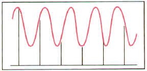
As you can see by the illustration, our example reproduced analog signal doesn�t look quite the same as the original one - it�s made up of a sequence of "steps". If you listened to the audio signal represented by the final waveform, it would be noticeably "raspy" and wouldn�t have the high fidelity of the original. The key to making the reproduced analog signal as identical as possible to the original one is to sample often enough (sample rate) and with enough possible "steps" (high enough resolution.)
For the sample rate, the calculation is easy. You must always sample with a rate at least twice as fast as the highest frequency you want to reproduce. This is called the Nyquist theorem. In the case of audio, for example, in which we can hear frequencies up to 20 kHz, the sampling rate must be at least 40,000 times a second. In fact, CDs have a sample rate of about 44 kHz, just to be sure we can reproduce everything we can hear.
If the Nyquist rule isn�t followed, and the sample rate isn�t high enough for the signal we�re trying to digitize, strange things happen when we try and reproduce the signal back to its analog form. In the accompanying pictures, notice that we have sampled a wave in the first figure (the vertical bars show us where we have picked our sample points.) But when we try to reproduce the signal based on our samples, we get a different wave altogether. This is because we haven�t sampled often enough for the high frequency of the original signal.
|
When good sampling...
|
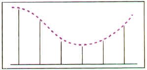
...goes bad!
|
For the resolution, more experimentation is needed. In the case of audio, we have found that 256 possible levels of voltage change (as the electrical audio wave moves up and down in level) are enough for decent audio resolution. This seems like a peculiar number - 256 - but because all of this digital world works with the computer binary system, it really isn�t all that odd. Its other name is "eight bit resolution" and is expressed mathematically as 28. This means that there are eight possible "0" and "1" combinations that could represent all the levels of change. Some people find that eight bit resolution isn�t enough (they can hear the digitization, the raspy distortion,) so they prefer to sample audio at 16 bits (216, or 65,536 possible levels.)
Analog to Digital Converters
|
The basic component in an electronic digital system is the analog-to-digital converter (ADC). It converts the voltage to be measured (an analog quantity) into a discrete number of pulses (a digital quantity) that can then be counted electronically. Analog signals are electrical voltage levels; a digital computer can only handle discrete bits of information. The A/D converter thus allows a physical system to be read directly by digital devices. The digital representations being converted to, are usually in the form of binary numbers, and an ADC's precision is given by the number of binary bits it can produce as output. For example, an eight-bit ADC will produce, from its analog input, a digital output that can have 256 levels (28).
|
Analog to digital converter ("counter" type)
|
A typical A/D converter is made from a register that can hold a digital value, an amplifier, and a voltage comparator. The register outputs are electrically summed to produce an electric current proportional to the digital value of the register. This current is amplified and compared to the unknown input analog signal. As long as there is a discernible difference, the register value changes one step at a time until there is no difference. Finally, the register holds the digital value equivalent to the analog input. This process is known as sampling. The faster the A/D converter can produce fresh samples, the more accurate will be the digital representation of the analog signal.
Digital to Analog Converters
|
Digital to analog converter ("resistive ladder" type)
|
A digital-to-analog converter, on the other hand, abbreviated as DAC, converts digital representations of numbers back into analog voltages or currents. DACs may be constructed in several ways, the simplest of which is called a weighted resistor network. In this kind of device, each incoming bit is used to apply a voltage to the end of a resistor. If the bit is "1", the voltage is high; otherwise the voltage is low. The resistances vary as powers of two, with the least significant bit being applied to the largest resistance. So, the maximum current flow into each resistor is proportional to the binary weight of the bit, and the total current flowing out of the resistors is proportional to the binary value of the input.
|
Digital Video
Why digital video? Why should we convert an analog signal (viewed with our "analog" human eyes) into a series of "1"s and "0"s? There are several reasons. Digital transmission and processing generates a minimum of degradation (if the signal is recovered properly) - a zero is a zero, and a one is a one, providing they're received anywhere within the range of where they should be. As a result, there is no problem with noise and other deterioration as with analog methods. Interfacing with computers and optical manipulation devices (e.g., DVEs, stillstores, frame synchronizers, paintboxes) becomes much easier if there aren't conversions to do from analog.
But First, A Word From Out Analog Video World...
In the analog videotape world, there are two types of recordings: composite and component.
Composite
Composite recording takes the full NTSC video signal (with its chrominance "layered" on top of the luminance), and attempts to put it down on tape. In the case of say, VHS videotape, the entire signal modulates a high-frequency FM carrier, and this carrier, in turn, magnetizes the videotape.
Sometimes the chrominance is separated from the luminance with filters, and these two elements are recorded by different processes. For example, in the case of VHS cassette recordings, the luminance is recorded with a much higher frequency FM signal than the chrominance (hence the name "colour under recording.")
Component
|
Component video
|
Betacam solves the problem of recording the NTSC signal by recording unencoded component signals (called Y, R-Y, B-Y), usually on two separate video tracks, one after the other. Remember the colour encoding process we mentioned a few chapters back? In component video, The R, G, and B information is mixed to create luminance (Y) information, and run through two balanced modulators to form R-Y and B-Y colour component information.
|
How Many Samples Does It Take?
Component Video
In the component world, we have Y (luminance), B-Y and R-Y. We sample the luminance signal at 13.5 MHz. This frequency was chosen because it affords a certain compatibility with NTSC and PAL digital video streams (yes, actual international agreement on a television standard.) The B-Y and R-Y information is sampled at only half this rate - 6.75 MHz - because, frankly, our eyes can't really discern colour detail much more closely than that. We learned that fact while developing NTSC back in the 1950s.
If you do the math, this gives us 858 luminance samples for the entire line of video, and 720 of these are for active video. For each chrominance component, the sampling is half as often - 429 samples for the whole line, and 360 for active video. We can sample video at either a 10-bit or 8-bit width.
For luminance, there will be only 877 discrete levels of video in the 10-bit system (you might expect 1024), and only 220 levels in the 8-bit system (instead of 256), as the remaining levels are reserved, as a safety margin.
Component serial video has special timing reference signals (TRS), and they are inserted after the leading edge of the horizontal sync pulses, during the conversion from analog to digital. Theses signals indicate within the serial bit stream the beginning and the end of the video lines and fields.
For the chrominance components, there will be only 897 discrete levels of video in the 10-bit system, and only 225 levels in the 8-bit system.
Ancillary data can be sent in lines 10-19 (and 273-282 in the second field), as well as vertical sync, horizontal sync, and equalizing pulses. Right now, only audio information has been standardized, but this means that audio (up to four channels of it) can be sent with video, down one coaxial cable.
Composite Video
So far we've been dealing with the component video serial transmission (it's got B-Y, Y, R-Y, Y all sequenced down one cable.) What if we've got composite video to begin with (which would be generated by much of our existing television plant)? NTSC composite video can be digitized too, but it's sampled at 14.31818 MHz, which is 4 times the frequency of colour subcarrier. If you do the math, this gives us 910 samples for the entire line of video, and 768 of these are for active video. We can sample composite video at either a 10-bit or 8-bit width. There will be only 1016 discrete levels of video in the 10-bit system, and only 254 levels in the 8-bit system, as the remaining levels are reserved. Also, when digitizing composite video, all of the video is digitized, including the blanking, sync signals, and colour burst. As in component serial video, composite serial has timing reference signals (TRS), and they are inserted after the leading edge of the horizontal sync pulses.
Also, as in component serial, ancillary data can be sent in lines 10-19 (and 273-282 in the second field), as well as vertical sync, horizontal sync, and equalizing pulses.
Let's Start Sending Those Digital Video Signals
So, we've figured out how to convert analog video into a digital format, and send that stream of information down a bunch of wires.
We can send it as a composite stream (14.31818 million samples per second).
We can also ship it as a component stream. These three signals will be interleaved in the following fashion:
and so on. You will notice that we always start the "stream" with a "B-Y" colour component, then a luminance component, then an "R-Y", and finally, another luminance. This sequence then repeats.
Let's see just how much information we're trying to cram down our coaxial cable. We have 13.5 million samples of luminance, 6.75 million samples of R-Y information, and another 6.75 million samples of B-Y information. If we were to send this, multiplexed, down a parallel transmission path, we would be sending 13.5 + 6.75 + 6.75 = 27 million samples per second.
But, we're sending this data stream down a serial coaxial cable, remember? Each sample has 10 individual bits of information (a "1" or "0"), so our actual transmission rate down a serial coaxial cable will be 270 million bits per second! If our samples are only 8 bits "wide", then our transmission rate lowers to 216 Mbits per second.
Back to the composite digital video signal for a moment. When we serially transmit our signal here, our 14.31818 million samples per second of composite video becomes 143 million bits per second in a 10-bit composite world. And here's a wrinkle: in the 8-bit composite world, the two "least significant bits", as they're called, are forced to a "0" state, so it still takes 143 Mbits/sec to transmit an 8-bit resolution composite serial digital signal.
|
Transmission Rate of Digital Video Signals
|
|
Format
|
Sampling Width
|
Parallel Transmission
|
Serial Transmission
|
|
Component
|
8
|
27 Mbps
|
216 Mbps
|
|
10
|
27 Mbps
|
270 Mbps
|
|
Composite
|
8
|
14.3 Mbps
|
143 Mbps
|
|
10
|
14.3 Mbps
|
143 Mbps
|
Sampling Rates
|
Various digital video sampling rates
|
We are now familiar with what 4:2:2 sampling is. What are the other ones we hear about? Here's a synopsis of the digital video formats:
4:2:2 - a component system. Four samples of luminance associated with 2 samples of R-Y, and 2 samples of B-Y. The luminance sampling rate is 13.5 MHz; colour component rates are 6.75 MHz. The highest resolution for studio component video. The active picture bit-rate is 167 MBps for 8-bit, and 209 MBps for 10-bit sampling.
4:4:4 - all three components are sampled at 13.5 MHz.
4:2:0 - this is like 4:2:2, but doing what's called "vertically subsampled chroma." This means that, while the luminance sampling rate is 13.5 MHz, and each component is still sampled at 6.75 MHz, only every other line is sampled for chrominance information.
4:1:1 - the luminance sample rate here is still 13.5 MHz, but the chrominance sample rate has dropped to 3.375 MHz. The active picture bit-rate for both 4:2:0 and 4:1:1 is 125 MBps.
|
It's Still Video: Synchronization Signals
There are a few more things we should mention about this serial transmission stream. Through this discussion of sampling video and turning it into a digital form, we've lost sight of the fact that it is video, and has a certain line length, synchronization pulses, and so forth, which we need to recover, or at least indicate the presence of, if we are to put this data back together as television pictures that we can view properly.
Each line of digitized video has two more parts - special time reference signals (TRS), which are called start of active video (SAV), and end of active video (EAV). The SAV and EAV words have a distinctive series of bytes within them (so they won't be mistaken for video information), and a "sync word" which identifies the video field (odd or even), and presence of the vertical blanking interval and horizontal blanking interval. The TRS signals are the digital equivalent of our analog sync and blanking.
Scrambling To Get It Together
Next, all of the conversions to "1"s and "0"s may have one real problem: it's possible that we may have a big string of all "1"s or all "0"s in a row. This is no small difficulty, since, in serial transmission, we want to see a lot of transitions so that we can recover the "clock", which is the constant time reference.
|
The solution to this problem lies in something called scrambled NRZI ("non-return to zero - change on 1") code ("NRZI" is pronounced "nar-zee.") The "non-return to zero" part means that, if we come across consecutive "1"s in a serial stream, the voltage remains constant and does not return to zero between each data bit. This is, of course, our problem situation. Scrambled NRZI, in turn, is derived by converting all the "1"s to a transition, and all "0"s to a non-transition.
The neat thing about this code is that it is polarity independent. This means that it's no longer a case of a "1" being a high voltage, and a "0" being a low voltage, but rather a transition indicates a "1", regardless of which way the transition is going! This means that the clock can be recovered more easily, and there's no confusion about what a "0" or "1" is, either.
|
Why we need NRZI
|
Weird Stuff
We've digitized the video, figured out the encoding, and we've pumped the signal down the coaxial cable. It should be perfect from here on, forever.
Or is it?
With good old analog video, you can send the signal a long way down a coaxial cable. If the signal starts to degrade, it loses colour and detail information, but this can be boosted somewhat with an equalizing DA, so things don't look quite as bad as they are.
|
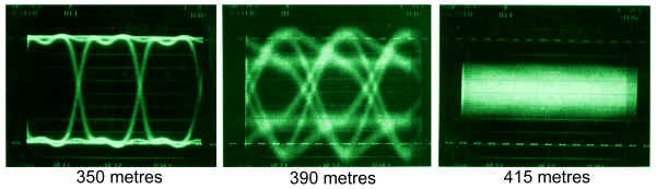
The problem with digital video is that the signal is excellent until you send it too far, at which point the signal is non-existent! The fall-off doesn't happen over hundreds of feet; it all plunges downhill over a critical 50 feet of cable.
We could probably live with one "hit" a minute, running our digital video 375 meters down the cable. We will get a glitch every second if we extend that cable only 10 more meters. We will get interference 30 times a second if we lengthen the cable another 10 meters. The graph is for a serial digital signal signal at 143 Mb/sec. The critical length is closer to 290 meters for a full 270 Mb/sec signal. At the critical length, a little more extension greatly increases the chances of fouling the signal. The solution to this is to capture the signal and regenerate it, fresh, every 250 meters or so. This is like jam-syncing time code - the code is read, and regenerated anew.
|
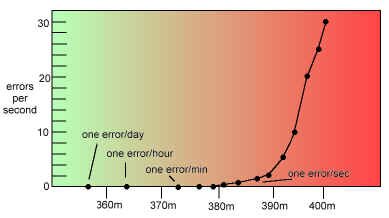
Graph showing "cliff effect" of serial digital transmission
|
The effect of different cables lengths on a serial digital signal (the "cliff effect")
Compression
So far, we've been content with sending our very high-speed digital video signals down the wire. In some cases, this involves up to 270 Mbits/sec. A lot of information is going down that cable.
This requires a fairly wide bandwidth transmission path, which is something that we do not always have available to us. Consider that the local cable company tries to cram dozens of signals down one coaxial cable (with varying degrees of success, admittedly). Even our standard television channel (with its 6 MHz bandwidth) can only handle about 25 Mbps. Most computer network interfaces are between 10 and 160 Mbps. A telephone company ATM (asynchronous transfer mode) line runs around 155 Mbps. Fibrechannel has a maximum rate of 100 Mbps. None of these transmission technologies are even near what we need for a full bandwidth digital transmission.
Let's look at this another way. A nice clean 4:2:2 digital component signal needs 97 Gigabytes of storage for a one hour show. Even composite digital video needs about 58 GBytes for an hour's programming. How big is your hard drive?
We need to reduce the bit rate, folks. Enter video compression.
Lossless or lossy?
Lossless compression...loses no data. This allows only small amounts of bit-rate reduction, say, a maximum of 3:1 - the information can only be compressed to a third of its original size.
Lossy compression, on the other hand...well...loses information. If you're careful with your mathematical formulas, you can make this almost invisible, but it isn't perfect. If you're not careful, however, things become quite messy. But, you can send the signal down a lower bandwidth channel.
The choice is yours.
Spatial Redundancy
|
|
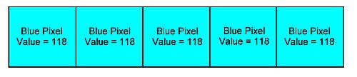
We can reduce the signal by looking closely at it. In any given frame of television, there is a probably a lot of redundant information - large areas of a single colour, for example.
|
If we can somehow encode the information so that, when we look at a blue sky, instead of saying:
BLUE PIXEL, BLUE PIXEL, BLUE PIXEL, BLUE PIXEL, BLUE PIXEL
we say
FIVE BLUE PIXELS
we can save a lot of transmission time and information repetition.
Temporal Redundancy
|

|
Also, if we look at frames of video shot before and after the frame we're encoding we might find that it's a static shot with no movement. In that case, we can save a lot of information by, instead of saying:
|
A VERY DETAILED FRAME OF VIDEO
A VERY DETAILED FRAME OF VIDEO
A VERY DETAILED FRAME OF VIDEO
A VERY DETAILED FRAME OF VIDEO
|

|
we can say
A VERY DETAILED FRAME OF VIDEO
IDENTICAL FRAME
IDENTICAL FRAME
IDENTICAL FRAME
|
Block Level Compression
We can also apply a technique that allows us to use a lower number of bits for information that occurs frequently (similar to the spatial redundancy theory described above, but instead of working on the video line or video frame level, it's done on a "small block of pixels" level.) This allows more difficult scenes to have more "headroom" as the bit stream moves along, so they won't be distorted.
A combination of all three methods can, with judicious use, reduce our 270 Mb/sec stream to 6 Mb/sec. There is some debate about whether this will be noticeable to the home viewer.
Compression Types
JPEG: This stands for Joint Photographic Experts Group and is a method for compressing still, full colour images.
Motion JPEG: a variation on the above, which is essentially a way to play back a bunch of JPEG images back-to-back. Sort of like a "flip book" animation.
MPEG: This is an acronym for Moving Pictures Experts Group, and is an international standard for moving pictures around. There are various versions of MPEG.
MPEG-1: This was the first MPEG standard (released in November, 1991), and is used with CD-ROMs for moving picture playback. This is referred to as the SIF format, with a frame size of 360 x 240 pixels. It has a VHS-like quality.
"MPEG-1.5": well, not really a standard. This is the application of MPEG-1 to full-size, interlaced, broadcast video. And it shows. There are noticeable artifacts in the video (sometimes disparagingly referred to as "pixel-vision" or "chiclet-vision".)
MPEG-2: This specification was issued in November, 1994, and is the full-motion, broadcast video version of MPEG. Many broadcasters have adopted it for their compression method.
|
MPEG-2 Profiles and Levels
|
|
Level
|
Profiles
|
|
Profile
|
Simple
|
Main
|
SNR
|
Spatial
|
High
|
4:2:2 Profile
|
|
Frame Type
|
I, P
|
I, P, B
|
I, P, B
|
I, P, B
|
I, P, B
|
I, P, B
|
|
Sampling
|
4:2:0
|
4:2:0
|
4:2:0
|
4:2:0
|
4:2:2
|
4:2:2
|
|
Scalability
|
non-scalable
|
non-scalable
|
SNR scalable
|
spatially scalable
|
SNR, spatially scalable
|
SNR, spatially scalable
|
|
High (e.g., HDTV)
|
Enhanced
|
|
1920 x 1152
60 fps
80 Mbps
|
|
|
1920 x 1152
60 fps
100 Mbps
|
|
|
Lower
|
|
|
|
|
960 x 576
30 fps
|
|
|
High-1440
|
Enhanced
|
|
1440 x 1152
60 fps
60 Mbps
|
|
1440 x 1152
60 fps
60 Mbps
|
1440 x 1152
60 fps
80 Mbps
|
|
|
Lower
|
|
|
|
720 x 576
30 fps
|
720 x 576
30 fps
|
|
|
Main (e.g., conventional TV)
|
Enhanced
|
720 x 576
30 fps
15 Mbps
|
720 x 576
30 fps
15 Mbps
(conventional television)
|
720 x 576
30 fps
15 Mbps
|
|
720 x 576
30 fps
20 Mbps
|
720 x 608
30 fps
50 Mbps
|
|
Lower
|
|
|
|
|
352 x 288
30 fps
|
|
|
Low (e.g., computer compressed)
|
Enhanced
|
|
352 x 288
30 fps
4 Mbps
|
352 x 288
30 fps
4 Mbps
|
|
|
|
|
Lower
|
|
|
|
|
|
|
MPEG-2 has a wide range of applications, bit rates, resolutions, qualities, and services. This makes it very flexible, but how do you tell your decoder box what you're doing? You build into the format a number of "subsets" specified by a "Profile" (the kind of compression tools you're using) and a "Level" (how complex your processing actually is.) MPEG-2 supports transport stream delivery (streaming video), high definition video, and 5.1 surround sound.
MPEG-3: was to be the next step, but its variations ended up being incorporated into the MPEG-2 standard, so this version was never released by the Group.
MPEG Audio Layer III (MP-3): This is a format for compressing audio at extremely low bit rates. Its real application is on the Internet for the transferral of audio, but not in real time. There have appeared on the market several software packages that allow playback of MP-3 audio on your computer. Hardware versions of the MP-3 player are about the size of a personal tape player, and download music selections from your computers, storing them in RAM for instant access.
MPEG-4: Released in 1998, this is a standard to allow reliable video compression at lower speeds of transmission (4800 bits per second to 64 Kb/s). This means the possibility of video transmission over telephone lines and cellphones, and high quality audio over the Internet. The starting point for full development of MPEG-4 is QuickTime, an existing format developed by Apple Computer, but the resulting file size with MPEG-4 is smaller.
MPEG-7: a "Multimedia Content Description Interface". Not necessarily a compression method, per se, but more a standard for descriptive content within compression. This type of information (above and beyond audio and video information) is called metadata, and will be associated with the content itself, as textual information, to allow fast and efficient searching for material that you're looking for.
MPEG-21: secure transmission of video and other content.
How MPEG Works
Given that there are spatial (adjacent pixels within a frame are similar) and temporal (the same pixel between sequential frames are similar) redundancies in video, we can do compression.
|
BEFORE: a graphical representation of a block of digitized pixels
|
In MPEG, a small block of pixels (8 x 8) is transformed into a block of frequency coefficients. What the heck are they?
In any given block of pixels, there will be some pixels that aren't that far off in video level from their neighbours. This is something that we can exploit in our compression scheme. What we do is perform a Discrete Cosine Transform (DCT) on the block of pixels.
|
AFTER: how Discrete Cosine Transform reduces the amount of information about the block of digitized video
|
Without getting into the math too much, we end up with an 8 x 8 block of information representing how large the changes are over the entire block of pixels, and how many different changes there are. These are what's called frequency coefficients. Now you know.
Because the block only has 64 pixels in it, and they're all right next to each other, and their values are probably pretty close to one another, most of the 64 "value spaces" available for the direct cosine transform calculation have values of zero! So, instead of sending 64 values for 64 pixels, we may end up sending only 10 or 20 values from the DCT array (the rest of them are zeros.) That�s DCT compression for you.
|
How a block of DCT coefficients are read
|
To further complicate this understanding of how DCT works, the value array is read in a zig-zag fashion, so that the likelihood of obtaining long strings of zeros is greater. A long string of zeros, in turn, is sent by a unique code word, which takes less time than sending a bunch of zeros back to back.
One of the neat things about the DCT process is that the compression factor can be determined by the values contained in what�s called a "normalization array", which is used in the actual DCT calculation. Change the array, and you can change the compression factor.
|
The DCT transform, as we've just gone through it, is used in both JPEG and MPEG compression systems.
What Makes MPEG Different?
JPEG is for stills; MPEG is for motion. With DCT, we've dealt with video on the single-frame level, but MPEG goes a step further. MPEG uses prediction. MPEG encoders store a series of frames together in digital memory, and have the ability to look "forward" and "backward" to see changes from one frame to the next.
Forward prediction uses information from previous frames to create a "best guess" for the frame we're working on. Backward prediction does the opposite - it uses information from frames "yet to come" and creates a "best guess" for the present frame. Bi-directional prediction is a combination of the two.
MPEG's frame stream has three kinds of frames within it: Intraframes (like a JPEG still); Prediction Frames (those predicted from Intraframes); and Bidirectional Frames (those predicted from both Intra Frames and Prediction Frames). You'll often see these frames referred to by their abbreviations: I, P, and B frames.
MPEG encoding and decoding
I-frames don't produce very much compression, after the DCT's been done on them. They are considered "anchor frames" for the MPEG system.
P-frames provide a bit more compression - they 're predicted from the I-frames.
B-frames provide a lot of compression, as they're predicted from the other two types of frames - they're totally derived from mathematics. If the math is accurate, they'll look just like the equivalent frames in full-motion NTSC video, once they�ve been decoded. If the math is not so good, artifacts will appear.
The whole bunch of I, P, and B frames together is called a group of pictures (GOP).
MPEG: Not For Everyone?
So, if MPEG is so great, why not use it not only for transmission, but for distribution everywhere, for in house production? Think of the bit-rates saved!
The answer lies in the way MPEG actually works. With all those I, P, and B frames running around, it's clear that you can't just cut over on your video switcher to a new video source anywhere. Nor can you edit MPEG easily, for the same reason. You only get a new group of pictures approximately every � second, which isn't often enough for those of us who are used to cutting to the nearest 1/30th of second. The only solution people have come up with so far is to decode the MPEG bitstream to digital video or NTSC, do your editing or cutting, and re-compress your creative output back again.
Cable and Satellite Transmission Compression
Now, all this talk of MPEG compression is not to be confused with "compression" terminology used with cable and satellite television transmission systems. That type of compression refers to the number of television signals that can be delivered with compression techniques. For example, a 4:1 compression on a satellite channel means that they are trying to squeeze four television signals on one transponder. However, to do this, they may use a 25:1 MPEG compression scheme on each channel!
What Is A Video Server?
|
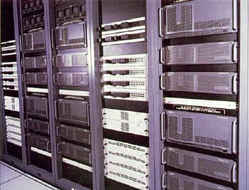
A group of video servers arranged in a system, incorporating many computer hard disk drives (courtesy Fox)
|
A server, in simple terms, is a system by which we can store large amounts of information and get at it fairly readily. An example of a "technologically light" server would be a tape librarian, a large room with many shelves to hold the videotapes, a card catalog or computer database...and a ladder. This system gives us mass storage, cross-referencing, and relatively immediate retrieval.
In our quest for faster and easier access to material, we developed computer controlled videotape server systems. The earliest broadcast TV video servers were analog quad VTR commercial spot players, first developed in the 1970s (e.g., Ampex ACR, RCA TCR.) Later versions have incorporated more modern tape formats, more VTRs per rack, and larger tape "shelf" storage capability (e.g., Sony Betacart, Flexicart, LMS.) Over the last several years, automated tape systems have incorporated digital videotape as their format.
|
Today, hard drives are capable of storing gigabytes of information on them, and with or without compression techniques, the viability of using this computer storage device for video is no longer in question. MPEG, Motion JPEG and other compression types allow the bit rate to be lowered to a speed that the hard drives can accept. Another frequently used solution is to "spread" the information to be recorded across several hard drives simultaneously, each drive taking a portion of the total bandwidth of the digital video signal.
One of the biggest concerns about computer hard drives is shared by all individuals who have had their personal computer's hard drive "crash" - what about online reliability? Fortunately, additional stability can be achieved by configuring groups of disk drives into various redundant arrays of independent disks (RAID) (also known as Redundant Array of Inexpensive Drives.). This adds error correction algorithms to the system, and with that comes the ability to swap out a defective drive from the array, without losing your video information. A fresh, blank drive is inserted in place of the faulty one, and the information can be "reconstructed" by the error correction and RAID software.
Optical drives are also being used in digital video servers, but for the most part, these drives are "write once read many" (WORM) systems. This means you can write the "master" of your commercial spot to this drive, and play it back as many times as you like, but the medium is non-rewriteable. Once the disk is full and the material on it is stale, it must be removed and replaced with a fresh disk.
Applications
|
Up until fairly recently, the central use of video server technology (of whatever type) was for commercial playback. One of the largest problems with integrating spots for air is the fact that there are several video sources required over a very short (two to three-minute) period. Before video servers, the solution to this was a large bank of videotape machines, loaded up separately by an operator, and rolled in sequence to make up the commercial break. Once the break was run, the entire bank of machines would be rewound, tapes stored, and a new series of spots would be laced up in time for the next break.
Machines were then invented that had one or two tape transports and some kind of a series of cartridges, each holding one commercial spot. In the beginning, these were based on two-inch quad videotape technology (see the accompanying photograph.)
|
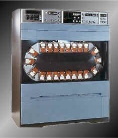
Early cart machine (courtesy Barry Mishkind www.oldradio.com)
|
The alternative to this is to make a "day tape," a reel with all of the commercial spots pre-edited for the day's broadcast. Master control then has only to run one videotape machine for each break. The day tape has the advantage of less machinery being tied up during the broadcast day, but late changes in commercial content cannot easily be accommodated. This application is natural for a video server.
A related application to commercial playback is the simple replacement of videotape machines. This is now done in large network establishments where repeating material is aired several times.
|
With increased demand (especially in news services) for several people to have access to the same clip of videotape, it is becoming more common to see news editing systems incorporating some kind of non-linear, hard drive based computer editing system. The process here involves the cameraperson shooting the raw footage and then having the final takes dumped into the non-linear editing server. This footage, in its digital form, can be viewed by the assignment editor, the reporter, the writer, the show producer, and of course, the on-line editor, all at once if necessary - these people can call it up on various workstations located around the newsroom. Depending on the workstation (or editing station) characteristics, the clips can be seen in different resolutions, frame rates and sizes, and qualities.
|
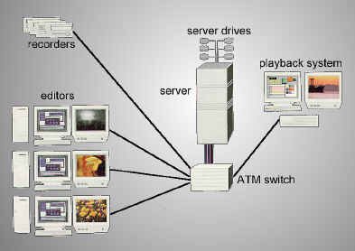
Typical news editing server system (courtesy Avid)
|
With the large longitudinal spread of Canada and the United States, a single satellite broadcast can appear in up to five time zones simultaneously. With material that may not be suitable for all audiences at once, separate "east-west" split feeds are becoming more and more common. Usually, a constant time delay (typically three hours) is all that's required. A video server (in its simplest form) is ideal for such a situation. The video information from the east feed is sent into the server, stored on the hard drives for three hours, and then automatically played out again for the west feed. The delay is continuous, with no worry about videotape machines having to be rewound, or breaking their tapes.
Cable TV companies are now offering "pay per view", which requires that the outlet have multiple program outputs of the same movie or special event, often with different starting times. Because hard drive video servers can have several outputs, even reading the same material seconds after one another, it's possible to "load in" one copy of a movie, and play it out simultaneously to many channels.
|

Thirty-two piece symphony orchestra, being played out from 32 different video servers simultaneously
|
With the proliferation of television channels either via DTV, digital cable, or direct broadcast satellite, there will be the desire to send to the viewer several different points of view of one scenario, whether it is a movie of the week or last week's football highlights. This type of parallel viewing is also convenient for editing suite situations where you have many different, but simultaneously recorded sources that need to be played out at once for an offline edit.
|
Almost all of these applications have incorporated into them a comprehensive file management system so that the various parties who have to work with the video files can do so effortlessly and quickly...and without a ladder.
Things To Think About:
In the analog world, time is continuously observed. In the digital world, time is sampled.
To convert our analog world to digital and back, we use analog-to-digital converters, and digital-to-analog converters.
Converting our analog video to digital has several advantages.
In order to convert analog video to digital, we must sample it.
How often, to what degree, and the method used depends on whether it�s composite or component video.
The samples of digitized video with their timing reference signals travel in a serial bitstream at a high rate of speed.
When sampling component video there are various standard sampling rates that can be used.
Serial digital video is scrambled so that the clocking signal may be more easily recovered.
Digital video has a very sharp "cliff effect."
There are various redundancies in video that we can exploit when we compress.
There are various compression methods that have been devised.
MPEG and JPEG use DCT compression techniques.
MPEG uses prediction to compress moving video.
Video servers are systems which can store large amounts of information and get at it quickly.
Video servers have various applications.
----------
Okay, if you really want to know, here's the formula:
Aren't you glad you were wondering about this??? (Back to where we left off in the text...)